Untitled Document

Any physical signal, i.e. the disturbance of an observable quantity that propagates in space and time, can be decomposed into waves. Familiar examples are water and sound waves, the former being associated with a variation of water level, the latter being associated with a travelling gradient of air pressure. Light is associated with an oscillation of the electromagnetic field that can be detected by the human optical apparatus. Notice that in the case of light there is nothing material that oscillates: just a physically measurable quantity (the field) that changes its value in time.

As long as their amplitudes are small, two waves in the same physical location don't interact with each other. This implies that when two or more waves are superimposed, the net wave displacement is just the algebraic sum of the displacements of the individual waves.

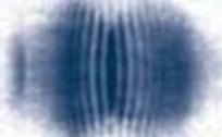
Since these displacements can be positive or negative, the net displacement can either be greater or smaller than the individual wave displacements. The former case is called constructive interference, while the latter is called destructive interference. Interference between the same two waves can be constructive at a given point O of space and destructive at another point O, depending on their phase relation at the two points (see figure 2). Therefore the signal's amplitude varies as a function of position in space, displaying a chessboard-like pattern that is the signature of interference.

To compare the behavior of particles and waves we consider a double-slit interferometer. The design of the set-up, which is based on an experiment carried out by Thomas Young 200 years ago, is showed in figure 3. Suppose first that we have a gun shooting a stream of bullets.

Now we repeat the same experiment replacing the gun with a source of monochromatic light and measuring light intensity instead of the number of bullets. Assuming that the relevant parameters are properly adjusted, the intensity distribution when the two slits are open displays interference fringes, i.e. alternate maxima and minima. At odds with the bullets experiment, here the total intensity distribution (green curve B) cannot be regarded as the algebraic sum of the independent contributions coming from each slit (red and blue curves). This result can be easily understood taking into account the wavelike nature of light and admitting that the wave emitted by the source is split in two secondary waves. Depending on their phase relation at each point of the detection plate, the two waves add up constructively or destructively, giving rise to alternate maxima and minima in the measured intensity. Figures 3 and 4 show the typical behaviors of classical particles (bullets) and classical waves in a double-slit experiment.

The bullets have to pass a filter with two vertical slits in order to impinge on the detection plate. Figure 5 shows various curves, representing, in different situations, the number of detected bullets as a function of the longitude x on the detection plate (because of the symmetries of the set-up, this is the only relevant coordinate). The red curve refers to a set-up in which only slit 1 is open while slit 2 is blocked. The blue curve refers instead to a set-up in which slit 2 is open and slit 1 is blocked. Green curve A is the distribution observed when both slits are open. As one expects based on elementary statistics, the green curve is just the (weighted) sum of the blue and the red ones.

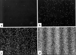
Now we come to atoms. If the same kind of experiment is performed using an atom beam, the result is not the one we get with bullets; rather, the distribution of the atoms detected at the detection plate displays interference fringes, as in the case of light (figure 4) !

One could conclude that this must be because atoms are actually waves. The problem with this conclusion is that regardless of the technique of detection employed, we always detect individual, well-localised spots, just as in the case of bullets. In fact, only when an ensemble of atoms has been recorded, interference fringes become apparent: ‘bright' fringes where a lot of individual atoms have impinged, ‘dark' fringes where no atoms have been recorded (see figure 7). The whole process looks as if the statistical behavior of the atoms were ruled by some wavelike law (see origins).

It's worth considering one more variant of the experiment. Let's suppose that our atoms are excited . This means that they are likely to decay to a lower energy level emitting a photon. We assume that the photon is emitted exactly while the atom is passing through the slits. In principle, the apparatus could be equipped with photon detectors allowing one to distinguish which slit the photon comes from. Thus we are now in a position of distinguishing (at least in principle) which slit the atom has passed through. Notice that this piece of information is essentially incompatible with the model associating to each atom two secondary waves (one for each slit). Surprisingly enough, when an ensemble of atoms is recorded in this configuration, interference fringes are not observed and the uniform distribution observed with bullets (figure 5A) is recovered. We get the impression that the possibility of monitoring the atoms' path forces them to behave like classical particles (see origins for further discussion).

Historically, the corpuscular nature of light became apparent before diffraction experiments with particles. In the early 20th century, the discvery of the photoelectric effect and of the Compton effect showed that, under some circumstances, photons and electrons scatter each other like billiard balls. Nowadays, single photons can be stored in superconducting cavities and manipulated by means of individual atoms, emphasizing at will either the wavelike or the corpuscular nature of light.